LuckGrib uses the Isochrone approach to solving the weather routing puzzle. For those who are interested in the deeper details, the isochrone algorithm is explained in more detail in the deep dive section.
Briefly - the weather routing problem can be described as:
- you start at a known position and time.
- you have a series of wind forecasts (GRIB files.)
- you have a destination you are heading towards.
- the system has a model describing how your vessel performs in various wind conditions.
As the forecasts involve complex wind patterns which are changing over time, you would like the system to find the fastest path from the start point to the destination.
Vessel performance - Polar diagrams.
The weather routing system needs a model for the vessels performance in various wind conditions. This is called a polar diagram, and is described in more detail elsewhere.
A polar diagram can be used to determine the vessels speed, given the true wind angle and speed (TWA, TWS.) For example, a sailboat will have different speeds if it is sailing close hauled, beam reaching or running with the wind.
Isochrones.
Starting at the beginning, if the vessel is at the start point, at the starting time, where could it be one hour later?
In order to solve this initial problem, the system will evaluate the wind forecast at the given point and time, and then send out a fleet of boats, in all directions, from the start point. Each boat in this fleet has a heading, and from that heading a wind angle can be calculated. Given this heading, wind angle and wind speed, the boat speed can be determined, from the polar diagram mentioned briefly above.
After this first iteration, you may see something like this:
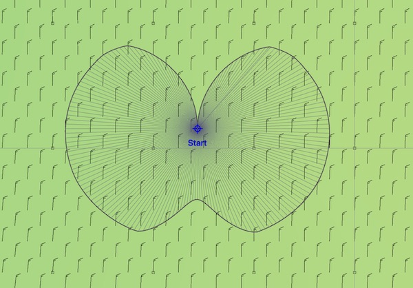
This represents the first isochrone in the weather routing solution. From the starting point, you could end up at any of the points on that outer line one hour later. The outer line, the isochrone, connects the points and represents where you could be after one hour of travel. Iso means constant, chrone is time - constant time.
The second, and all following, generations of isochrones are created as follows:
For each point on the isochrone, send out a fleet of boats. Collect this fleet of boats and find the ones which represent the maximum amount of outward travel, in all directions. The line connecting all of these best travel boats is the next isochrone. Repeat this process until one of the boats arrives at the target point.
Here is the isochrone solution after three generations:
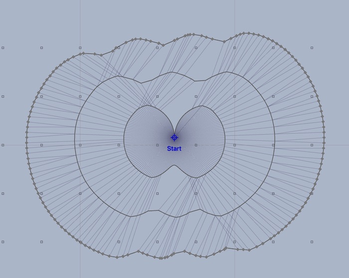
Note that this boat is faster sailing on a beam reach than upwind or downwind. This is reflected in the shape of the isochrones as they are extending further to the west and east than to the north and south (as there are north winds for this example.)
There are isochrones and isochrone segments being shown. The isochrones are the darker, radial lines. The segments are the paths from one isochrone point to where it came from on the previous generation. Keeping track of these segments is how the system finds paths through weather systems.
Isochrones are optimal solutions (but not unique.)
Each isochrone is built using what the algorithm considers the best positions, among the large collection of candidate fleet points. The positions which travel the furthest outward. The isochrone represents the maximum distance you can travel from the previous generation. There are many slower paths that can be taken, but these are not represented in this solution.
When the collections of isochrones, the isochrone solution space, arrives at the destination we can find the fastest path back to the start point by following the isochrone segments from one point to its previous point, following segment after segment.
Note that while isochrones represent optimal solutions, there is no claim that they are the unique optimal solution. There will most likely be alternate paths that can arrive at around the same time. However, none should arrive sooner.
The isochrone solution space.
The full set of isochrones in a weather routing solution is referred to as the solution space. The solution space is simply, all of the possible paths which were found by the isochrone algorithm, starting at the start point and time, radiating out in all directions.
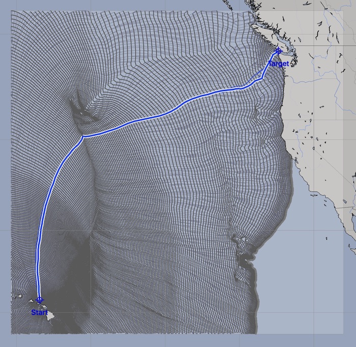
The path shown is the fastest path found between the starting point and target point.