I realize that this page is a little technical in parts. However, understanding this material may be useful in understanding the weather routing results and how to interpret them.

If you are not interested in this level of detail, simply skip onto the next page.

The problem of finding the optimum route, from one point to another, through a weather system is an interesting one. You start at a given position and time and want to end up somewhere else. How would you create a computer algorithm to solve the problem?

There are a few crucial pieces of this puzzle.

1. you need a way to evaluate the weather forecast at a given time and position to yield the wind vector.
2. you need a way of estimating the vessel speed given the forecast wind.
3. you need a way to project a point forward in time to where it could be, given its heading and speed.
4. you need a way to organize all of the generated projections in some manner which makes sense.

The first point is something that LuckGrib excels at. LuckGrib’s weather file interpolation across space and through time is second to none.

The second point is solved using something called a Polar Diagram, and is described in more detail elsewhere. As with the weather, LuckGrib uses sophisticated interpolation techniques when evaluating the polar diagram.

The third and fourth points are the main topic of this article.

How to start?

To simplify the problem, the algorithm will step through the forecasts at a certain time interval. Since we know where we are at the start point, the next step is to find out where we could be a little while later. For example, if we start sailing at noon, where could we be 20 minutes later?

Here is one possible result for this first problem:

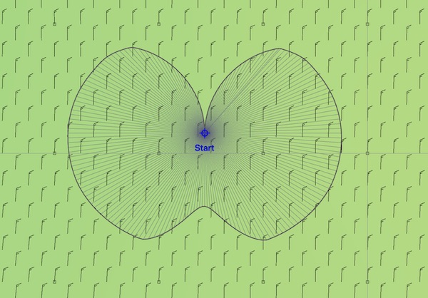
We start, of course, at the start point. Then we evaluate the wind from the GRIB file. In this case the wind is from the north at 16 kts. With the wind speed and direction, we can estimate the boat speed as it sails at different angles to the wind, and given these boat speeds and headings, we know where the fleet of boats, which is sent out from the start point, can end up. The picture above shows 180 new positions, which are the locations where you can end up from the start point after 20 minutes. Note that the positions directly into the wind do not travel very far, as a sailboat can not sail into the wind. Close hauled, close reaching, beam reaching, broad reaching and running are all represented. (Later you will see how to exclude impossible sailing angles from the set of possibilities considered.)

Brute force.

This first generation of positions is easy. The next generation is where things start to become difficult.

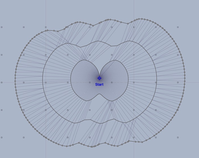
Given these 180 new possible boat positions, if you were at any of them, where could you end up 20 minutes later?

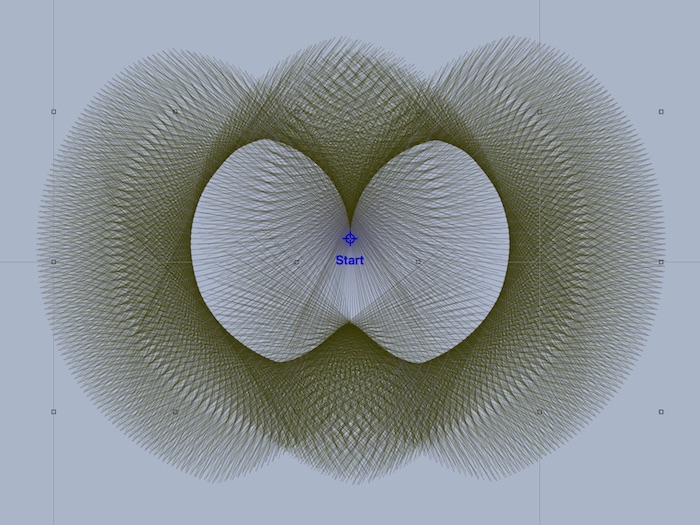
Things are getting a little more complex now. For each of the 180 points, the wind was evaluated and 30 new boats were sent out. There are now 180 * 30 = 5,400 positions shown. This is where things get interesting.

An example algorithm encoding this approach is something like:

time_interval = 1 hour (or whatever)
while we have not arrived:
    for every point from the previous generation:
        wind = evaluate_wind_field (point, current_time)
        for every heading leaving that point:
            boat speed = speed_from_polar (heading, wind)
            generate a new position for <heading, boat speed>
    arrived = did one of the new points hit the target?
    current_time = current_time + time_interval

If this process of sending out, on average, 30 new boats for each of the previous points was continued, we would quickly run out of, well, everything. This is called an exponential process. The formula for how many positions are in a single generation is:

number of positions = 180 * 30 * 30 * 30 …
number of positions = 180 * 30ⁿ

where n is the generation number.

For ocean passages, it is not unusual for the weather router to require 150 to 200 generations of this algorithm to arrive. The brute force algorithm described so far would require a lot of points. Returning to the formula estimating the number of positions required, here are some estimates:

30⁵ = 24,300,000
30¹⁰ = 590,490,000,000,000
30²⁰ = 348,678,440,100,000,000,000,000,000,000
30³⁰ = 205,891,132,094,649,000,000,000,000,000,000,000,000,000,000
30¹⁵⁰ = 3.67 x 10²²¹

These numbers become so large they are essentially infinite. No computer could solve this brute force problem, ever. Its not just a matter of waiting a few moments, the weather routing problem is impossible using brute force.

We need ways to simplify this problem.

Enter Isochrones.

Consider the image above again. There are a lot of positions that have been generated, but you can see that only a few of them push the boundary and extend the maximum amount from the previous generation. Many of the positions end up in the middle of the pack somewhere.

We are interested in generating optimal routes, or the fastest paths between two points. The set of points that are most interesting in the image above are the points which have made the most progress, the points which expand the envelope, or enlarge the amount of space covered.

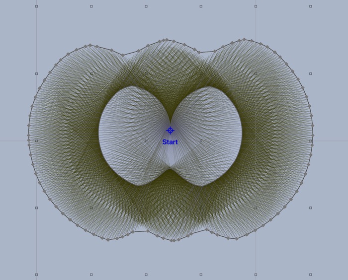
In the image above, the set of points which expands the maximum amount from the previous generation has been found, and connected together. The line connecting all of these points is called an isochrone.

An isochrone is a line representing constant time. In this example, all of the points on that isochrone can be reached at 40 minutes after the start time.

The brute force algorithm had 5,400 points in its second generation - this isochrone has around 90 points. The problem is no longer exponential. Generating isochrones changes the problem from being impossibly complex (exponential) to solvable in a reasonable amount of time.

The isochrones are representative of the best progress the entire fleet could make. Not all of the points close to the isochrone are in it - if we do not simplify the problem we end up with it growing too large to solve in a reasonable amount of time.

The set of points that occupy one isochrone are used in the generation of the next isochrone. As before, for each point on the new isochrone, the wind field is evaluated, a fleet of boats sent out at a range of headings, and all of the new candidate boats are collected. Finally, a new isochrone, which expands the maximum amount, is again created:

Normally, all of the points which were considered but not used in the generation of the next isochrone are hidden:

This type of isochrone image is what you will see in LuckGrib. The isochrone lines represent a connected set of points which can all be reached at the same point in time.

The line segments which connect a point on an isochrone to the point it was generated from are an essential part of the algorithm. For any point on an isochrone, the system knows the path that was used to arrive there.

Isochrone paths.

This process of generating new isochrones from the previous generation, each time trying to expand the space as much as possible, is repeated, over and over. Finally, an isochrone will move beyond your target point and the process will halt. At that point, the isochrone point closest to your target point is used to generate a path. This point on the final isochrone knows where it came from, and that point knows where it came from, all the way back to the start point.

Also, note from the dense set of candidate positions presented in some of the images above, that boats from different starting points can end up close together in the candidate fleet of positions. The algorithm will always choose the position which it considers the best, but wouldn’t it be useful to know that there were other positions close by which were just about as good?

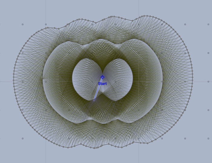
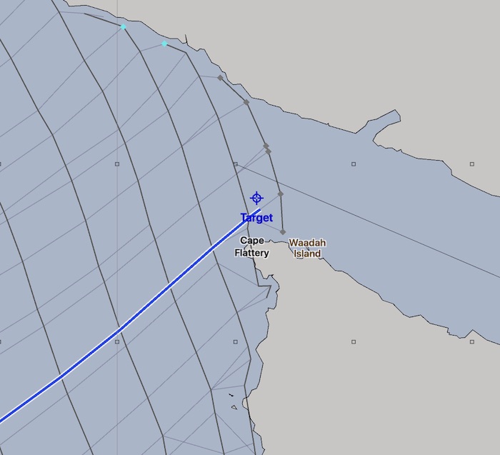
These close positions are recorded by the system and are shown as alterate paths:

The highlit path, the one with the white outline, is the optimal path found. The paths which are close to optimal are also shown. This indicates to you that there are close solutions in these areas. Close paths indicate less sensitive areas.

Isochrone algorithms. The same, but different.

Remember from the discussion on the Brute Force problem above that there is no way to solve this weather routing problem without simplifying the problem in a variety of ways.

Everybody who implements an algorithm to create weather routing solutions will have encoded a variety of decisions on how they approach the problem. Ways to reduce the problem from impossibly complex to something manageable.

Each isochrone weather routing algorithm will be different from all others. Many times, the different algorithms will come to similar solutions, but not always. If two applications use the isochrone approach in solving weather routing, do not assume that they generate the same results. There is a lot of variability among the different applications.

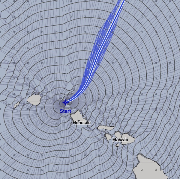
Isochrone solution space.

The term solution space refers to the entire set of isochrones that have been generated. For every point in this solution space, the application can find an optimum path back to the start point.