There are two types of weather models available:
- deterministic. Examples of deterministic models are: GFS, ECMWF, GDPS/GEM, HRRR, NAM, Icon, and many others.
- ensemble (or blends.)
In a deterministic weather model, the weather model creates a series of forecasts which it believes are the most likely. However, there is only a single set of forecasts. This is the models best attempt at a solution.
Deterministic models are generally pretty good for the first few days, and then later in the forecast their uncertainty grows and grows.
Ensemble and blend weather models accept that there is uncertainty present and generate their results by processing many variations of the deterministic models. It is generally accepted that ensemble models are more skillful for longer range forecasts.
There are two global ensemble models available in LuckGrib: GEFS (GFS ensemble) and the Canadian CMC ensemble. There are also a number of blend models, called the National Blend of Models (NBM). One of the NBM models, NBM Oceanic, covers an interesting portion of the Pacific and Atlantic and contains probability winds. (NBM Oceanic is discussed a little later.)
Just as shown in the previous example, where LuckGrib was able to create weather routing solutions using both 10m winds and wind gust information, LuckGrib is able to create solutions using an ensemble model. Recall that the wind/wind gust solutions used the same wind direction but different wind speed in their calculations. When using an ensemble weather model, each wind field contains both wind speed and direction. You will end up with a wider range of possible solutions using an ensemble model than when using any single deterministic model.
GEFS ensemble.
Using the same example as from the previous section, here are two routes using the GFS ensemble model:
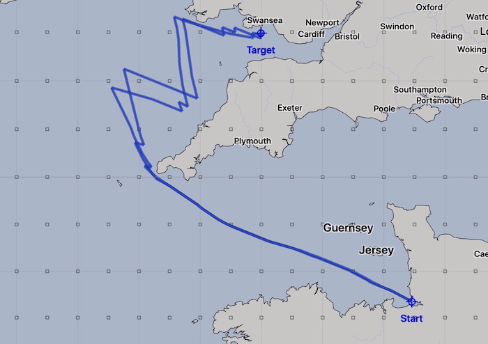
These two paths are a pretty close match to the prior example. They are again similar for the initial paths up to around Cornwall, and then differ in the final upwind portion. However, their durations and winds encountered are quite similar.
Full GEFS ensemble.
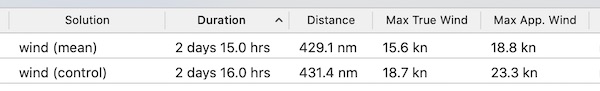
LuckGrib provides access to the full GEFS ensemble, the GEFS Ensemble with all surface wind members. The GEFS ensemble generates 30 different wind variations, which, along with the original control member and the average of all of them (the mean) results in a wide range of potential outcomes.

The image above shows an outlier in the initial portion of this passage, the path shown which is initially the most northerly. The weather in this stray wind field is initialy quite a lot lighter than the others, and the solver is having the boat head north to improve its angle to the wind (and generate more boat speed.)
The majority of these 22 wind fields are quite similar for the initial portion of this trip, and then after the Cornwall turn, there is a wide range of possibilities.
All of the paths make an arrival at the destination. All of the maximum winds encountered look quite reasonable. If I was considering a departure for this passage, that looks quite reasonable.
Ensemble models are increasingly useful when considering longer passages. Here are two more examples, between Los Angeles and Puerto Vallarta.


There are 22 weather routing paths shown in those images, and they are surprisingly in pretty close agreement. The first couple of days for the passages in each direction agree closely. As the passages progress, you would download fresh weather data and update your solutions.
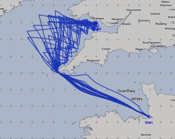
Here are two examples from Hawaii to Neah Bay. Note that this departure is on March 2nd. North Pacific weather systems at that time of year can be pretty inhospitable and full of uncertainty.
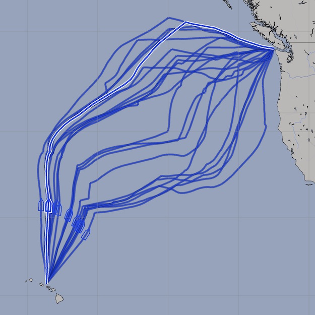
The route using the GEFS control winds, on the left, roughly corresponds to GFS. The mean (average) winds, on the right, is the average among all 21 members.
Reading the two images above - there is a great deal of uncertainty present. If you had created a solution using only GFS, you may not have seen this level of uncertainty. Which path would you follow? The best path is perhaps the path that has you remaining comfortably at anchor in Hawaii until this weather settles down a little?
If you had to leave on that passage, which direction would you head? Which of these 22 paths would you follow? This is where your good judgement and general knowledge comes into play. The weather routing system has alerted you to a huge amount of uncertainty. You could follow a general rule of thumb route, which would be to head north and later turn east. The mean winds path, on the right, may be a good choice for an initial path. (The better choice may be to wait.)
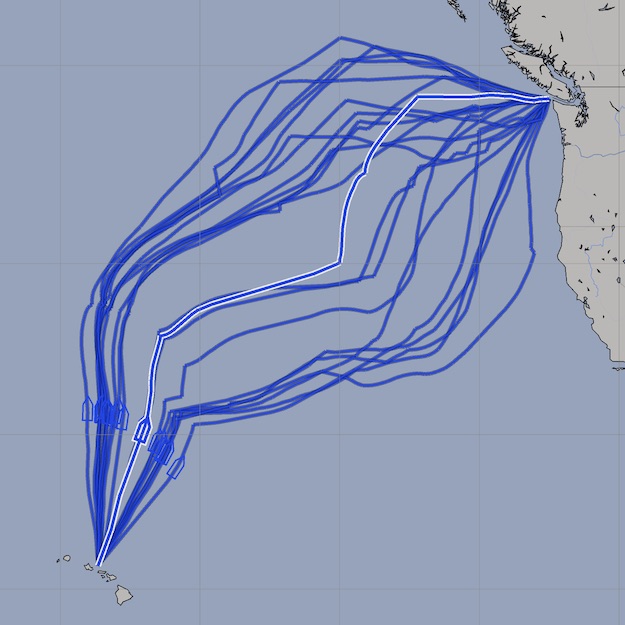
With the same weather file, running the reverse route, Neah Bay to Hawaii results in a much closer set of solutions:
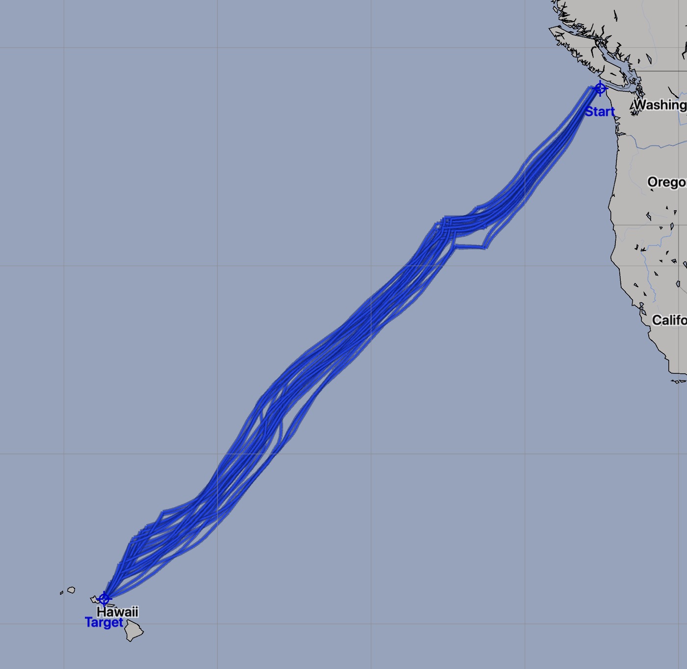
The image on the left is for a fast race boat, the Transpac 52. Faster passages allow you to reduce the uncertainty you encounter along the forecast (as the shorter passages mean you travel in the portion of the forecast which has less uncertainty.)
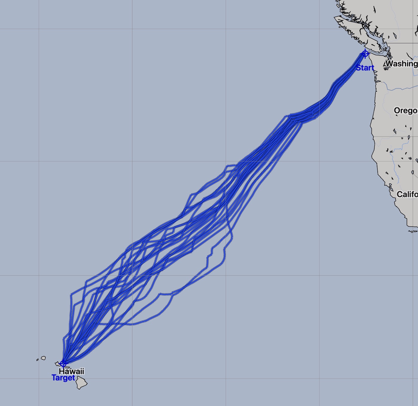
The image on the right is for a cruising boat which had an average passage speed of around 7 knots. As the slower boat took from between 12 ½ to 15 days, it used parts of the weather forecast which have great uncertainty, and the routes generated reflect this.
Even though the image on the right is showing a large spread of solutions, they all generally agree for the first three days. This is a good result. For the start of this passage, and the first few days, it looks like there is good agreement from this full ensemble weather model for a general path to follow. As you will be downloading fresh data daily, you will be able to update the paths along the way, making decisions on day three and beyond when you have access to better data.