The isochrone Weather Routing algorithm is an excellent method for finding an optimized path through a weather system between two points.
If you examine the results of the algorithm, you will notice that it never moves backward. The algorithm is always expanding the isochrone solution space, growing larger and larger. The algorithm stops when the destination is reached, the entire space has been filled or the process runs out of forecast data.
(The algorithm is described in more detail elsehwere.)
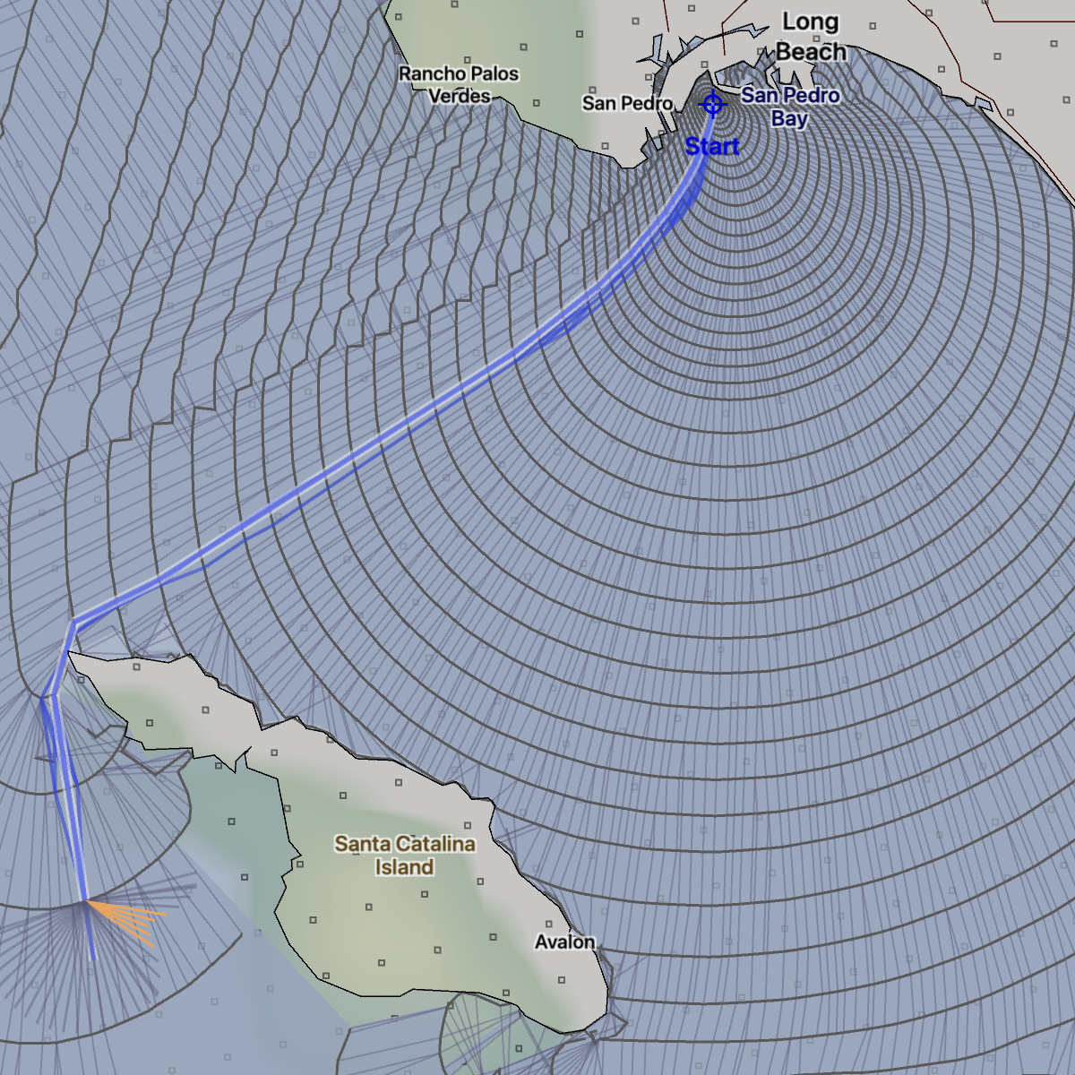 Los Angeles to Catalina.
Consider a route, where you want to leave Los Angeles, sail around Catalina, and then return back to Los Angeles. The first attempt at solving this route has a start point defined and has asked the solver to generate its full solution space. Note that the WR solver has traveled in both directions around Catalina island.
What is needed for this route is to describe to the solver that you want to go around the island and return to the mainland. This can be done by adding a constraint point which directs the solver to leave the island to port.
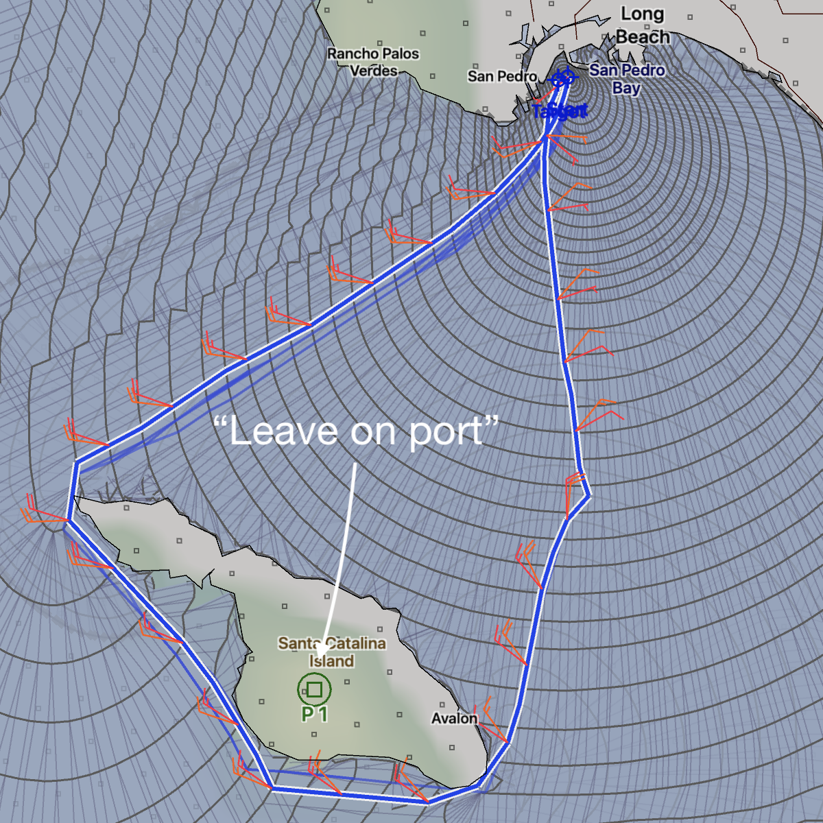 LA to LA, rounding Catalina on port.
If I do say so myself, this is pretty awesome. As far as I know, LuckGrib is the only isochronal WR solver which is able to accept these general point constraints.
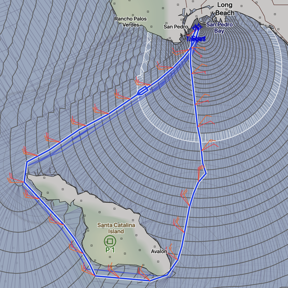
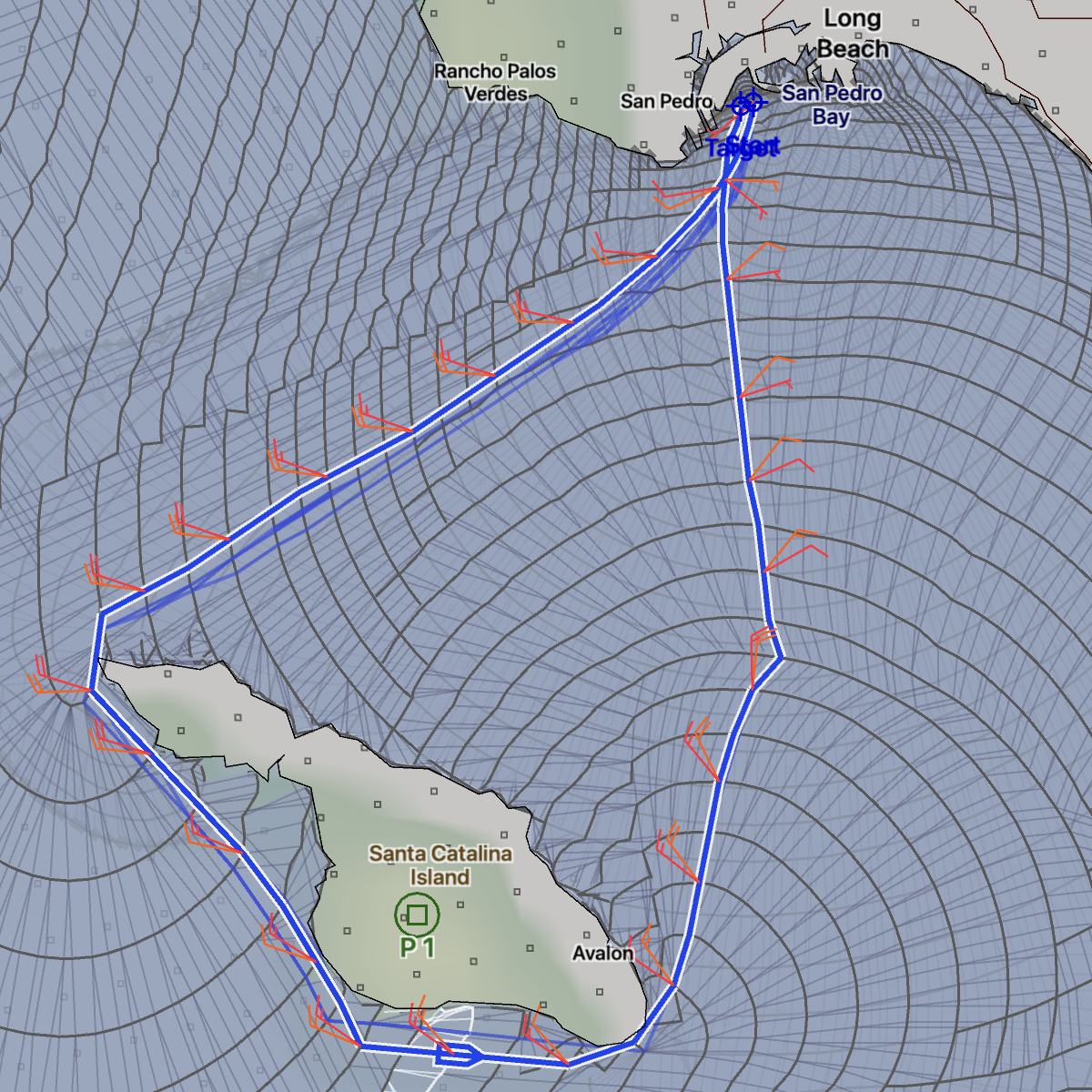
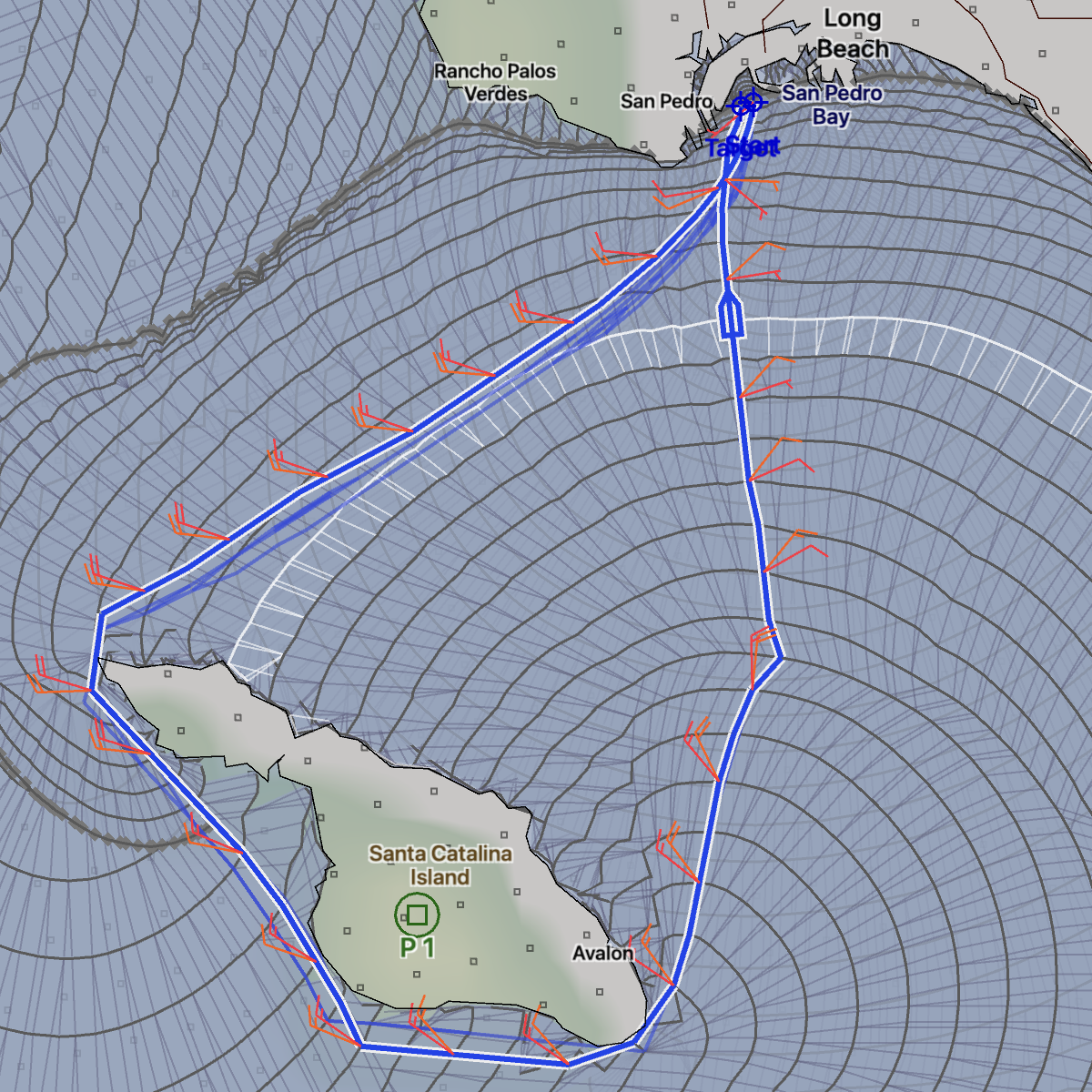
The LuckGrib solver is able to create an organization of the isochrone points such that the isochrones from a later time step are allowed to overlap the isochrones from an earlier time step, allowing the solver to find an optimized path from a large set of possible routes. The algorithm was enormously complicated to design and implement. Luckily, it’s very easy to use, and it remains a very high performance and accurate system.
In the image above, note that isochrones generated from the start point radiate out in all directions, attempting to round Catalina from both sides. As the isochrones start to approach the constraint point, on Catalina, they start to organize themselves into those vessels which satisfy the constraint and those that do not. The final image is showing the isochrone shape as the destination is approached.
Well, enough patting myself on the back. How can these new constraints be used?
Strategic route direction
Recall the discussion about the full GEFS ensemble from the Introduction | Uncertainty | Ensemble section. A route was shown between Hawaii and Neah Bay, at a time of year when the North Pacific ocean is generally inhospitable. The routes generated exhibited a great deal of uncertainty.
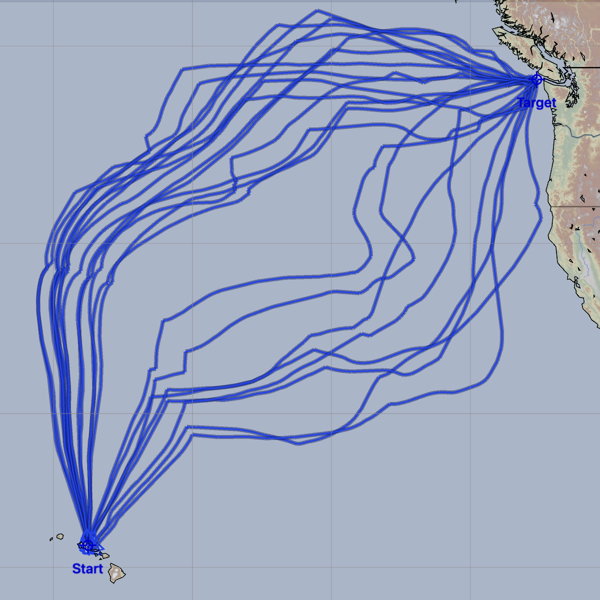
There is a general rule of thumb for this passage, that you head generally north and then turn east when you are somewhere around the latitude of Neah Bay. Many of the routes in the left image do not follow that strategy.
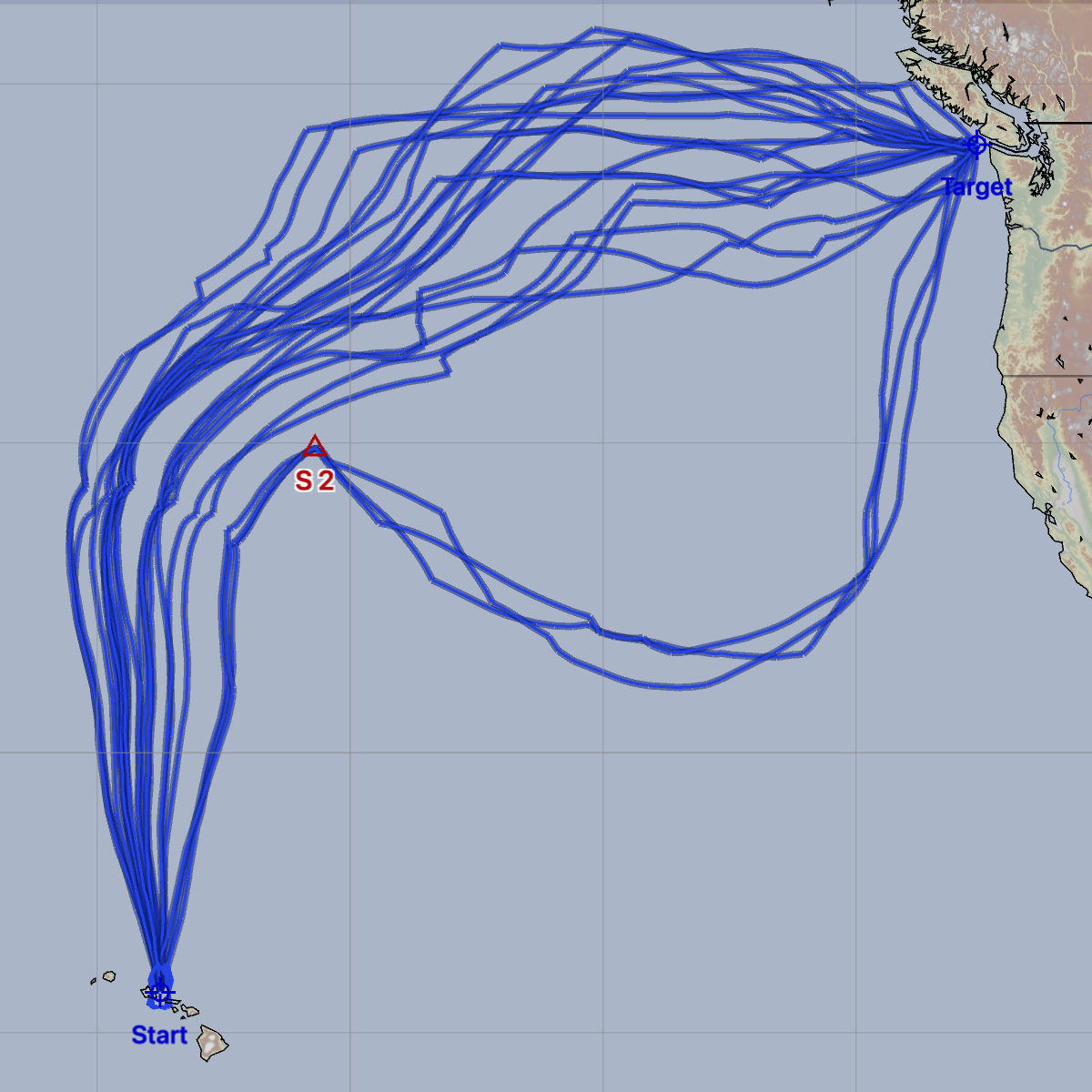
By creating a single constraint point, you can remove all paths which take the more southerly route, forcing them north. This is not advice on making this passage, but it provides one more demonstration for how constraints can be used to direct the solver to consider some paths and ignore others.
Note that three of the routes on the right, do leave the point to starboard, but then immediately head south again. The weather systems those paths are moving through appear to be quite inhospitatal to the northern route. Examining the solutions may lead to understanding what makes a good weather system to travel in, which may help during the departure planning for this passage.
Here is one final example, a passage from the Vava’u island group of Tonga, to the Bay of Islands, New Zealand. A rule of thumb for this passage is to try to cross 30° south somewhere north of New Zealand. This is meant to give you more options as the weather south of this latitude can change quite quickly. There is also an interesting option in this route, which is to stop at Minerva Reef, a beautiful tropical reef.
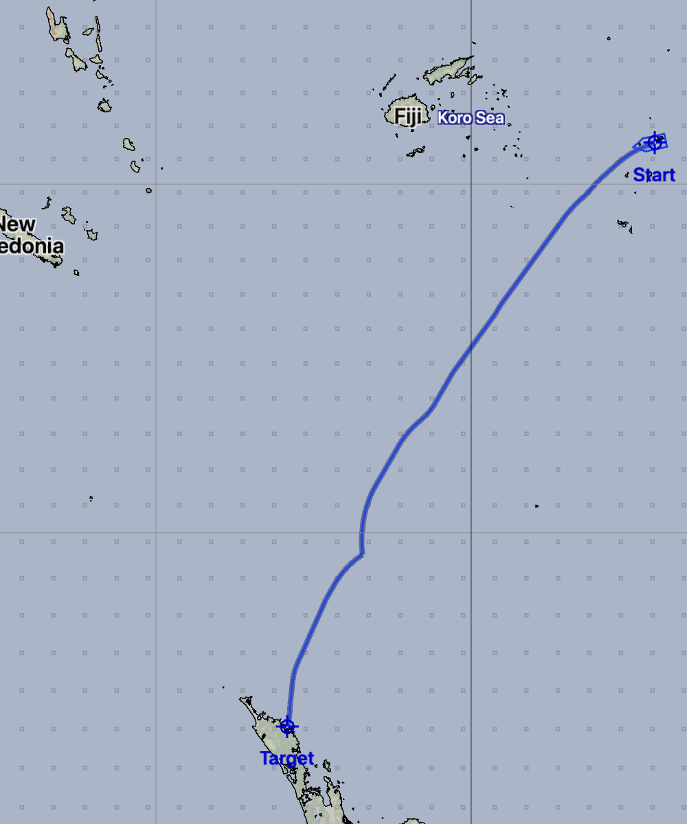
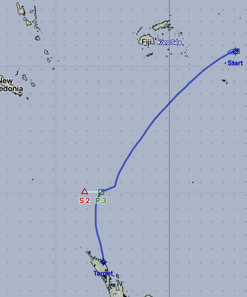
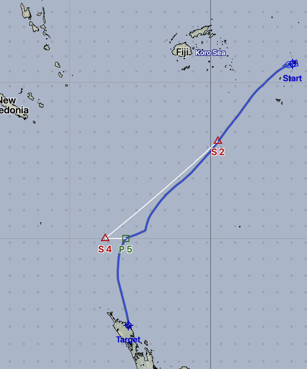
A gate can be described by putting a point on one side of it and marking it as leave to port, and then creating a second point and marking it as leave to starboard.
The unconstrained route takes 10 days 2 hours. The route passing through the gate takes 10 days 16 hours. In this example, there is no additional penalty for the route which also passes close to Minerva.
In this example, the spread of routes is pretty small. Choosing the option that gives additional navigation options seems warranted, as there is very little penalty for it.
It takes over 7 days to reach 30° with this vessel, and there is a lot of uncertainty in this weather forecast once you go further than three or four days. As you sail this passage, you will be updating your weather forecasts at least daily, and generating new routes as you make progress. As you progress, the penalty for taking a route through the gate may increase when compared to the more direct route.
Creating constraint sequences on a Mac.
This is described in more detail in the user manual.
Briefly, to create a constraint sequence, you use the Points and Routes tool:

Click down on the map in the area where you want the start of the boundary to be created. When the menu appears, select Create Constraint Sequence.
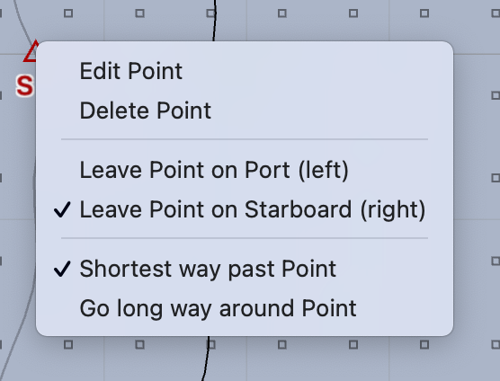
Each point can be marked leave to port or leave to starboard. To do this, either double click on a point, or control-click on the point. When the menu appears, choose the side you want the point left on. Depending on how the various points are oriented, you may also want to specify that the system go the long way around a point. This is discussed in more detail in the manual section.
Additional point constraints can be created by clicking on the map at a point you want to add, and then, from the menu, select Add constraint to sequence.
Any of the constraint points can be moved by clicking and dragging on them.
You can insert new constraints in a sequence inbetween two others by clicking on the line between them and choosing Insert Constraint from the menu. Deleting points, or an entire sequence, is done the same way (click on it, select the appropriate menu item.)
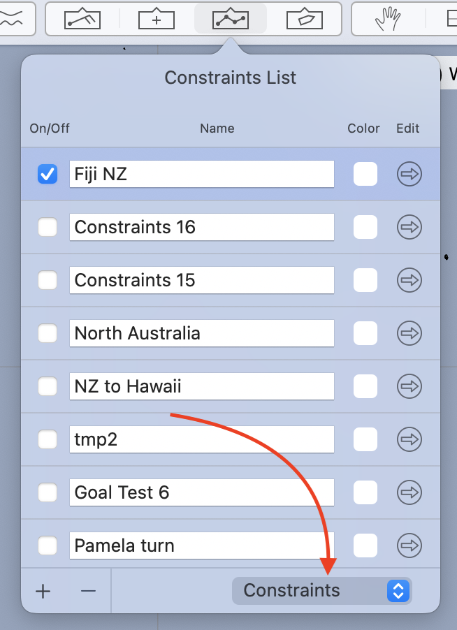
You can manage constraint sequences through the Routes List. Note that you need to choose Constraints, from the menu at the bottom of the lister:
After creating a constraint sequence, you can have a vessel use it by opening the vessel settings in the Weather Routing pane and setting the constraint sequence setting to the proper sequence.
Creating constraint sequences on iPad or iPhone.
There is a Routes and Boundaries tool, available in the tool area:
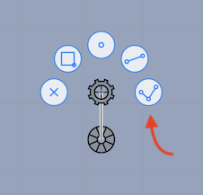
When that tool has been selected, you are able to create and edit constraint sequences.
The Routes and Boundaries tool is described in more detail, in the manual, but briefly, the buttons allow you to create routes, boundaries, constraint sequences, add points to them, move points, delete points and view some information about them.
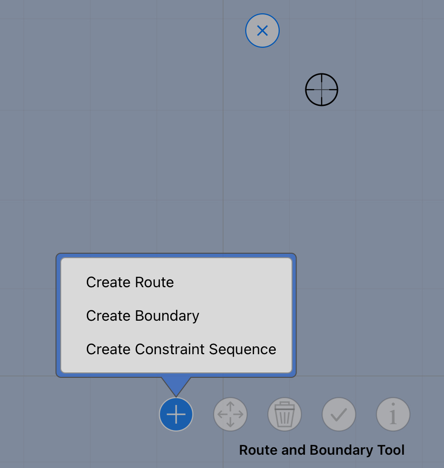
Once a sequence has been created, scroll the map to the second points location and append a new point to the sequence already started. Continue this until the sequence has been defined.
Each point can be marked leave to port or leave to starboard. To do this, move the central cursor over the point and tap the i button. A menu will appear, such as this:

Choose the side you want the point left on. Depending on how the various points are oriented, you may also want to specify that the system go the long way around a point. This is discussed in more detail in the manual section.
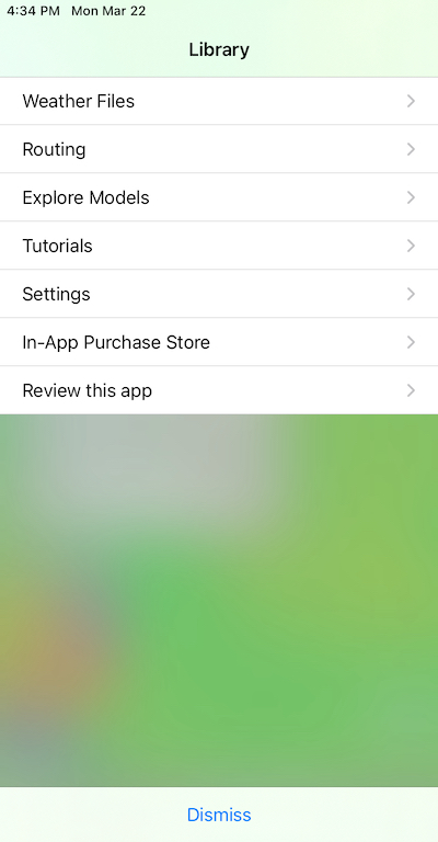
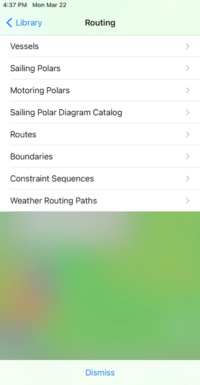
You can manage constraint sequences through the Routing area in the sidebar:
Associate the constraints with the vessel.
After creating a constraint sequence, you can have a vessel use it by opening the vessel settings in the Weather Routing pane and setting the constraint sequence setting to the proper sequence.
This is described in more detail in the user manual.