(These setting are enabled through the application preferences.)
Recall that isochrones are built from a large collection of possible positions and segments that are generated from the previous isochrone. For each point on the previous isochrone, a fleet of boats is sent out in all directions. As part of the isochrone generation, the algorithm will choose what it considers to be the best set of candidates, the ones that represent the maximum outward travel from the previous isochrone.
In this process of building isochrones, the isochrone creation algorithm will often encounter more than one point in the same local area. The algorithm chooses what it thinks of as the best point, and is then able to record the close candidates. These close points can be shown as alternative paths, and when there are a lot of alternatives shown, the algorithm is showing that there are alternate ways to achieve your objective.
How close is close?
This setting gives you control over what the algorithm considers to be a close point. By default, if a point is within 5% of the travel distance of the best point, it is considered close. You can make this value larger, to show more alternatives, or smaller, to show fewer. Setting the value to zero, or disabling it, causes the algorithm to not show alternate paths.
During this discussion, note that paths are always built from their end towards the start point. Given a end point, we know the optimum segment indicating where it came from. We may also have several non-optimum segments recorded at each point. Each time a non-optimum segment is traversed, the path is reduced by a small amount from being the best path possible.
Characterizing how much longer a passage along an alternate path is, can be difficult. The 5% close tolerance is used at each decision point (choosing the best segment the point originates from, or one of the alternate non-optimum points,) and overall, how much longer an alternate path is depends on how many non-optimum segments it is composed of. For example, it is possible that an alternate path used a single non-optimum segment, and other than that one, all of the remaining segments represent the best possible path back to the starting point.
Examples of different settings.

This vessel has a 2 minute tack / jibe penalty set.
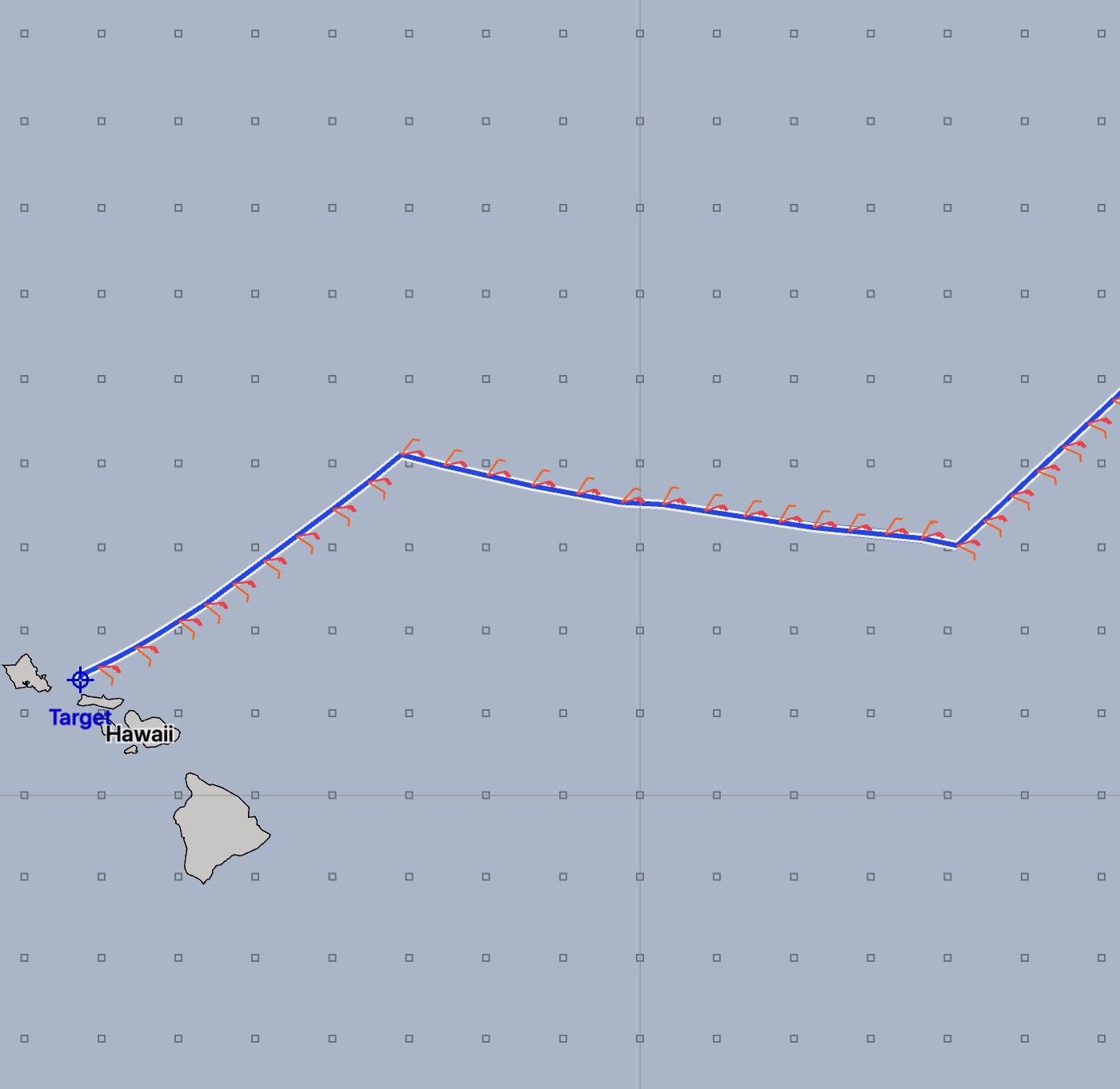
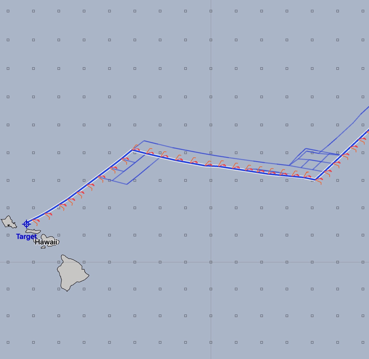
This example is for the final downwind portion of a passage to Hawaii, in trade wind conditions. The only setting which has been changed in each image is the close path setting. In each case, the solver has produced the same optimized path.
As can be seen, there may be close alternatives to the timing of the jibes.