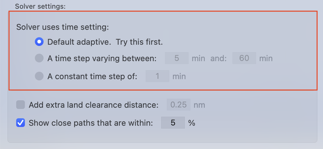
(These setting are enabled through the application preferences.)
Default adaptive, the automatic time step.
When the default adaptive setting is enabled, which is encouraged, the solver uses a sophisticated method of automatically choosing an appropriate isochrone time interval, based on a number of factors.
Without going into great detail, the solver starts with an initial time interval which varies from between 5 and 20 minutes, depending on how close to land your starting point is. As the algorithm progresses, if the solver is encountering a lot of land intersections, it may choose to keep the time increment small. If the solver finds itself sailing in open waters then it starts to slowly increase the time step.
Generally, the maximum isochrone interval the solver chooses, using the default adaptive method, is 2 hours.
As the solver sees that it is starting to approach the target point, it will start to reduce its time step. This has the effect of generating additional isochrone points, which will generate more accurate arrival information.
A varying time step.
This method is similar to the default adaptive method, with the addition that you provide the maximum and minimum time values. The solver will start a solution using the minimum value, and then as the solution progresses, based on a number of factors, the solver will slowly increase the step up to the maximum allowed.
Similar to the default adaptive method, if the route is hitting a lot of land intersections, it will increase the time step more slowly, or not at all. Also, as the solution approaches the target point, the time step is slowly reduced again, in order to generate a more accurate arrival.
Note that using this method with a minimum value of 20 minutes and a maximum value of 2 hours is close to, but not identical to the default adaptive method. The default adaptive method has additional heuristics it uses in its selection of the time steps that this method does not.
You may want to choose this method if you are sailing in congested waters, such as when close to land, or on an inland lake. If your routes tend to be short, and in areas with a lot of land intersections, choosing a shorter time interval may improve the ability of the solver to navigate around islands, bays, harbors and points of land.
You are encouraged to try the default adaptive method first, but if that is causing an issue, then give this method a try.
There is an example of this method, below.
A constant time step.
If you have a preference for generating all the isochrones at a single, fixed, uniform time interval then you can enable this setting and specify the interval.
One situation where you may want to set a fixed, small time increment, is if you are comparing the results of the LuckGrib WR solver to another system. Although, be aware that the results generated by LuckGrib may not be as good when using a fixed time interval. The automatic time increment method can produce superior results compared to a fixed time interval.
When comparing results between WR systems, you will likely want to do the comparison in LuckGrib, importing the other systems results via GPX files. LuckGrib has features which make doing the comparison easier than when doing it in other apps.
Open ocean time step example.
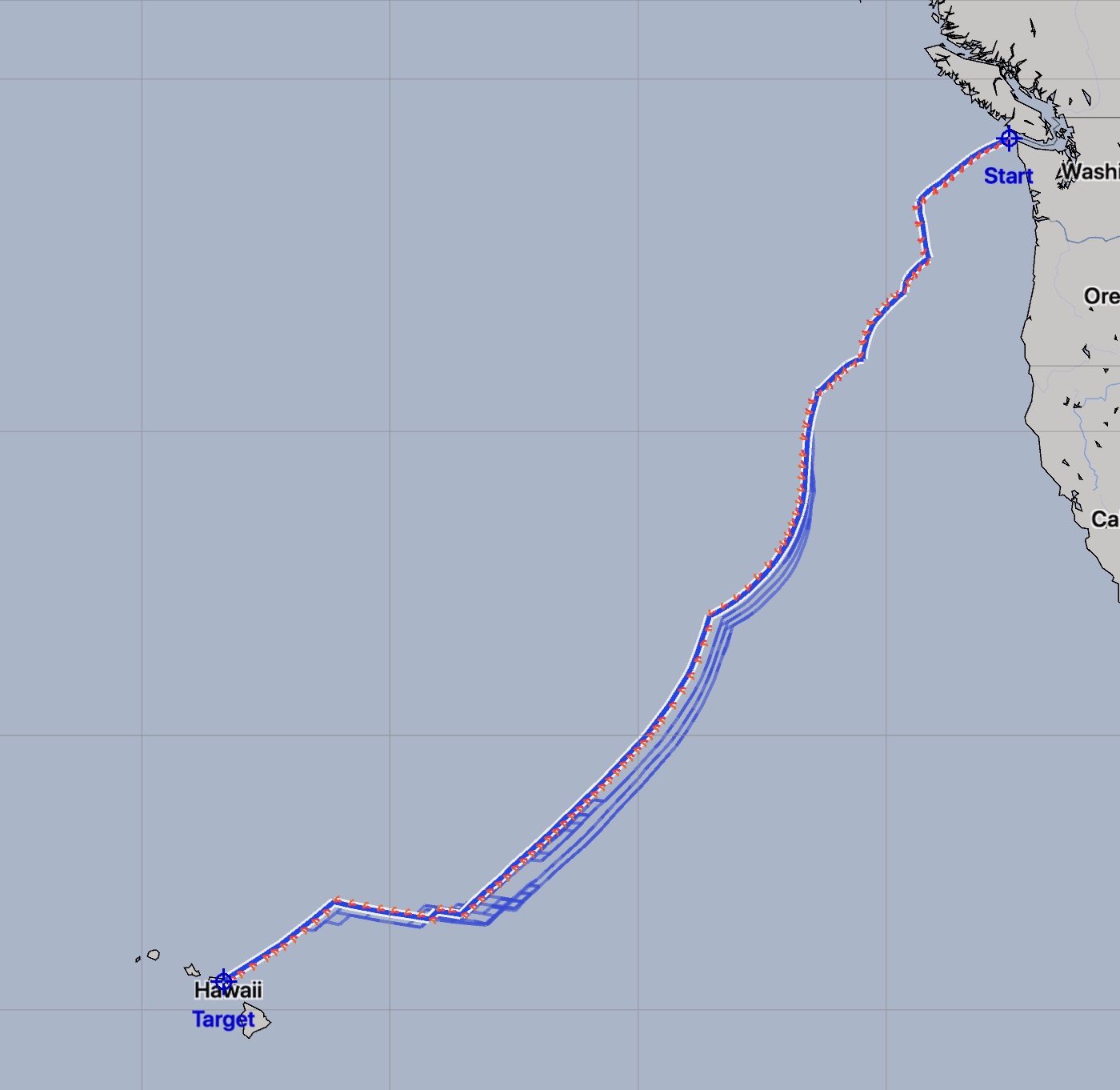
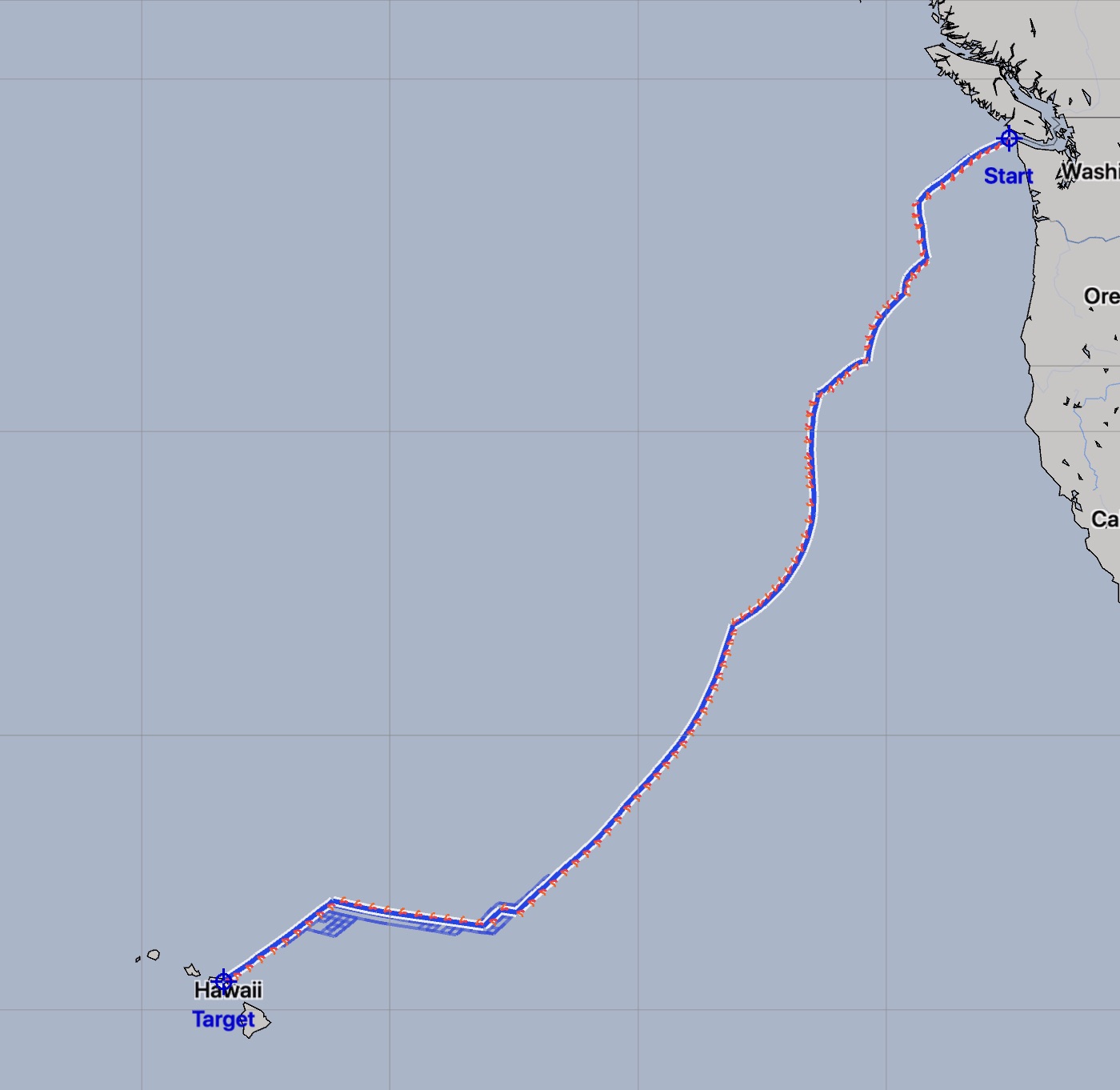

In this example open ocean passage, there are three paths generated, each with a different time step, and they are all essentially the same. The time duration of the paths are, from left to right: 8 days 8.6 hours, 8 days 8.8 hours, 8 days 8.8 hours.
The largest difference between these three examples is the amount of time taken to compute the solution. On a 2017 13” Macbook Pro, the average of three runs for these examples is: 0.588 sec, 0.890 sec and 2.95 sec. (If you have experiences with a different weather routing system, how does its performance compare for these examples?)
The author recommends using the default adaptive time step, and only change away from it if an issue arises - as discussed in this next example.
Constrained waters example.
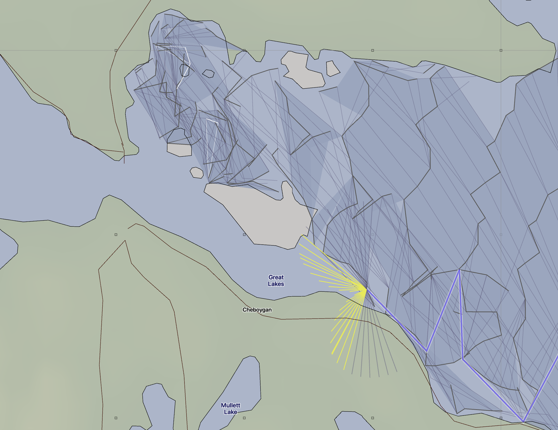
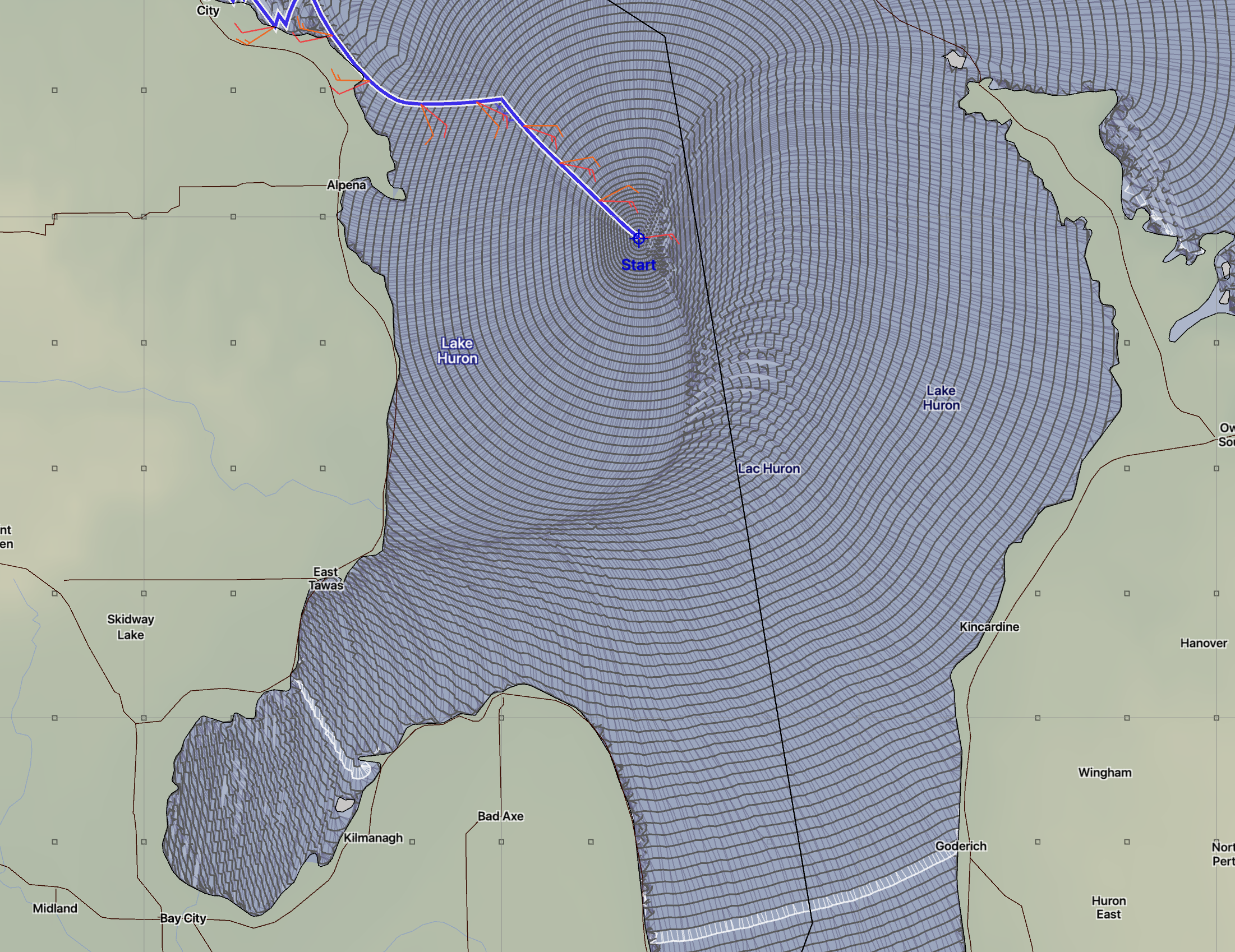
This is a somewhat contrived example, but shows a case of where the customized varying time step option would be useful. This example has the start point placed near the middle of Lake Huron, over 30nm from land. The solver considers this start point to be unconstrained by land, and so will choose a starting time interval of roughly 20 minutes. However, the size of the time increment by the time the solution approaches these more constrained waters, is larger than desired.
The main point of the left image is to emphasize the size of the isochrone segments in relation to the local geography. The segment lines are too large, which is interfering with the solvers ability to navigate around the islands.
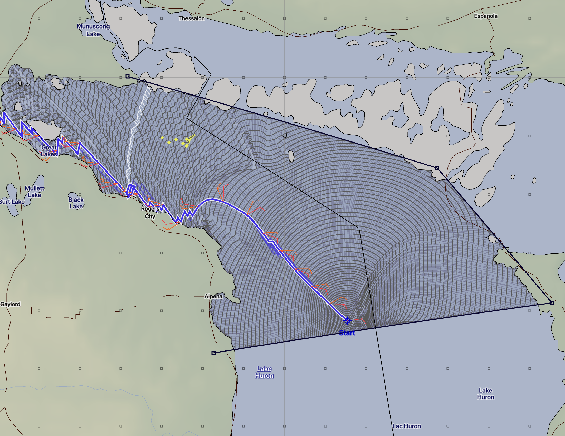
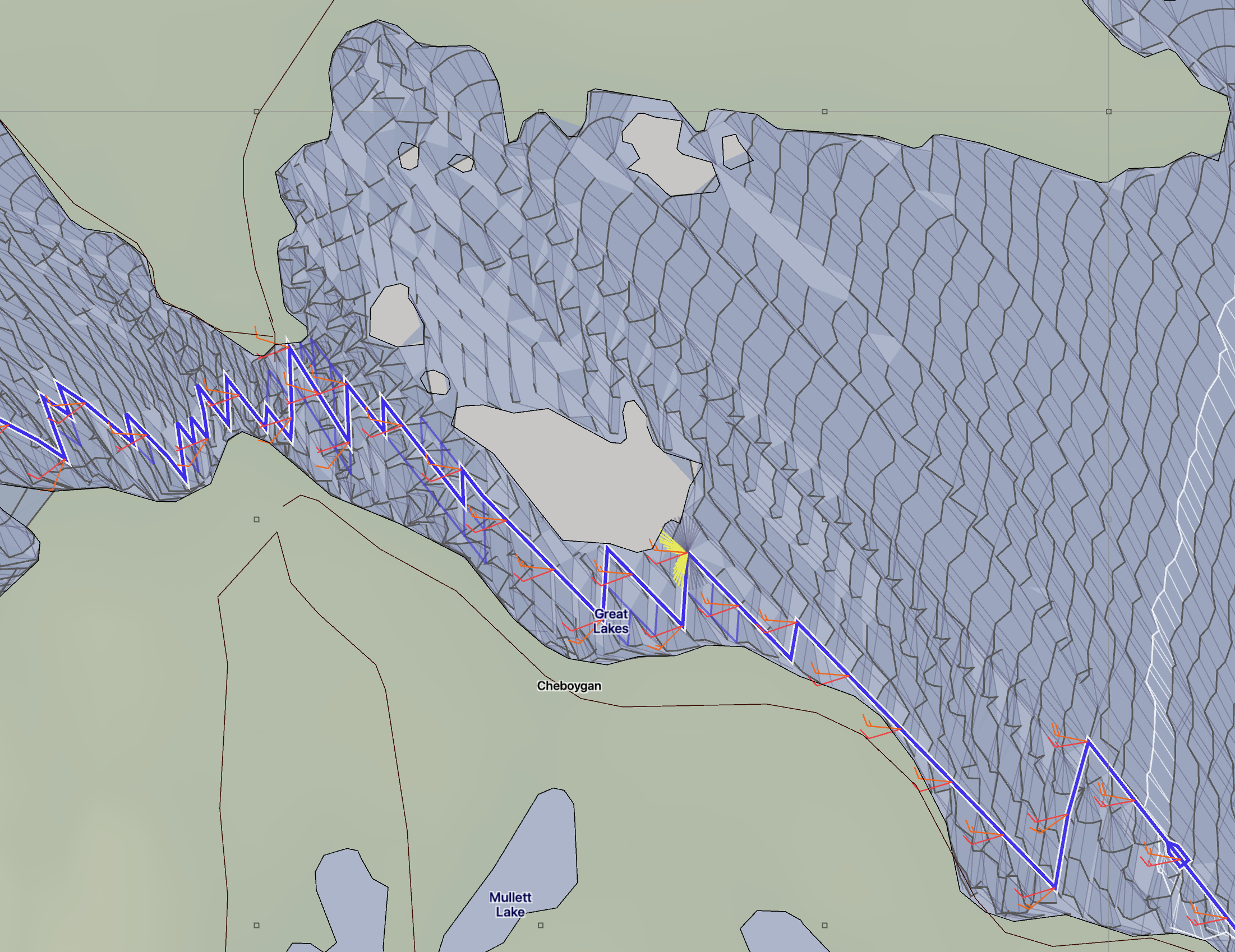
In the second example, on the right, a customized time range was given as starting at 5 minutes with a maximum of 20. The time step in the region shown is around 10 minutes. These isochrone segment lengths are much shorter, allowing the solver to create arrangements of them which navigate through these waters.
Note that when you force the solver to use these short time intervals, it is doing so along the entire solution space it is creating to find a path to the target. In this case, this means the solver is expanding the solution space to the south in Lake Huron and into other areas we are not interested in for this trip.
This expanded, fine grained solution space can consume a lot of memory and will slow the solver down in finding its solutions. If this becomes an issue, you can create a few boundary lines to chop off areas you are not interested in.